


Database design is the foundation on which we can build a successful initiative for maintenance and scalability. Administrators have the ability to maintain indexing, statistics, integrity checks and so on, but if a database is designed extremely poorly, even the tasks of indexing or maintaining statistics accurately, becomes very difficult. In some cases, the database is all but lost and a redesign initiative is needed, costly massive expenses.
When considering a database design, thinking of performance such as, how would this be indexed, in mind. While maintaining that thought process, also keep in mind the type of design that is being created. Historically, OLTP and OLAP are the high level designs to choose from. OLTP being a highly transactional or insert/update/delete, database design while OLAP, retains a wide table concept and de-normalized approach due to highly readable and little changes made.
In order to ascertain which of these designs required, there are two simple questions to ask.
These two questions are truly one and the same. The first, OLTP or OLAP, dictates the second. In an OLTP situation, what we’ll talk about today, normalization is going to effectively be critical to the performance we will have. On the same side, OLAP designed database can suffer drastically from a deeply normalized design due to the movement from high write to high read events. With the normalization being so critical, the first stage in that is to meet some level of normalization in an OLTP situation. If situations do present themselves where normalization has become a performance problem due to read/write variations, de-normalization can be effective.
Normalization is the standard process of reducing redundancy in a database. Although there are many levels of normalization, called normalized form, we’re going to focus on a simplistic level of normalization and a secondary level or 2NF for the example shown in this article. In this state of normalization, we will still see a high benefit in performance enhancements.
In the following two table structures, an ordering system was needed. Both table structures meet the needs of an order header, details and shipment storage. As shown in figure 1, the non-normalized structure has the word “poor” in the naming convention.
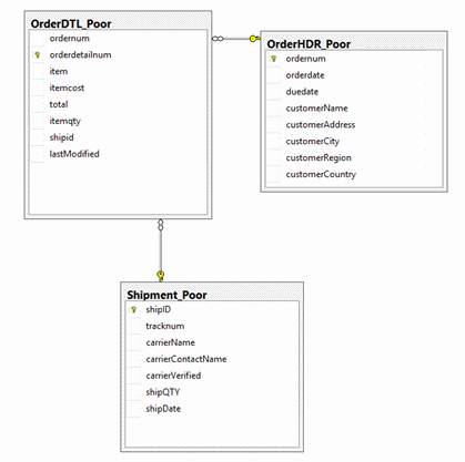
Figure 1 – Poor design showing lack of normalization
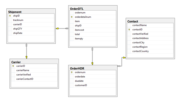
Figure 2 – Better design moving to normalizing levels
Both designs have been preloaded with 116,000 header rows, 4.2 million detail rows and 10,000 shipment rows. In the second, normalized structure, the Contact and Carrier tables are retaining data for 2000 contacts and 1000 carriers.
The basic view of redundancy
While designing, it is important to take the step of preloading expected data into your design. This data is completely volatile, but valuable from the aspect of seeing where redundancy can occur. Take the following queries:
SELECT TOP 1000 * FROM OrderHDR_Poor
SELECT TOP 1000 * FROM OrderHDR

In the results above, we can see that the data in customerAddress, customerCity, customerRegion, and customerCountry is repeated. This is a key indicator that normalizing the data is needed. This has been done in the second structure shown in figure 2 with Contact and further with Carrier.
Internal Structure Effects
Internally, these designs also affect storage. Since the designs are similar and the tables are relatively small, you may thing normalization isn’t needed. Normalization relates to performance, though. Some of the poor designs lead to inability to enhance performance with features available due to growth or scalability. Take a simple tuning effort such as the disk subsystems. A common standard is to locate files of different read and write needs on differently configured disks. In another simplistic example, allocating tables to specific physical disk heads can have a major increase on overall performance. Given the poor design in Figure 1, we have few options to effectively perform some of these methods to increase performance For example, if we rarely update customer addresses but insert a high number of order headers, we would want order headers to be located on a highly writable disk configuration, with the address data on cheaper, slower disk.
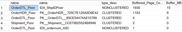
Another aspect to look at is how the design is affecting the overall page storage needs. Setting data types aside, the normalization level will have a direct effect on how many pages are needed. In both designs, we can use catalog views to look at how this impacts page counts.
select
    obj.name,
    idx.name,
    all_units.type_desc,
    all_units.total_pages
from sys.objects obj
  inner join sys.partitions parts on obj.object_id = parts.object_id
  inner join sys.allocation_units all_units on all_units.container_id = parts.hobt_id
  inner join sys.indexes idx on parts.index_id = idx.index_id and obj.object_id = idx.object_id
where obj.type = 'U' and obj.name <> 'sysdiagrams'
order by obj.name
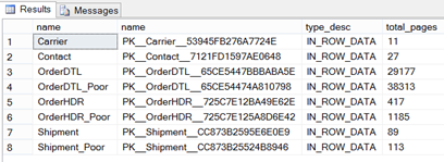
Figure 3 – Reviewing pages with catalog views
Although this information may not seem useful initially, it is critical to the performance of the database and what will be needed to satisfy the needs of both reads and writes in the database. The amount of data is exactly the same while one design has been normalized and the other has not been. We can see that the normalized design is consuming 29,721 pages (based on the data volume discussed earlier) and with the non-normalized design using 39,611pages, or an increase in storage needs of 30%.
Looking at Query Basics
Querying data that is not normalized has a few concerns and performance aspects that should be taken into consideration. The first is, querying data is faster when you have less need for joining tables. In a normalized design, joining tables is required. As you normalize to higher forms, more joins may be needed. Although this isn’t a new concept, you will still see a performance increase from simple queries from a normalized factor over the non-normalized design due to the overall page counts pulled into the buffer or, memory.
Take the example below and the plan generated from the query
CREATE PROCEDURE [dbo].[select_OrderDetailsByOrderNum] (@ordernum INT)
AS
SELECT
	hdr.ordernum,
	hdr.orderdate,
	dtl.item,
	dtl.itemcost,
	dtl.itemqty,
	CASE WHEN ship.ShipID IS NULL THEN 'Not Shipped'
	ELSE CAST(shipDate AS VARCHAR(12)) END [Ship Date]
FROM OrderHDR_Poor hdr
JOIN OrderDTL_Poor dtl ON hdr.ordernum = dtl.ordernum
LEFT JOIN Shipment_Poor ship ON dtl.ShipID = ship.shipID
WHERE hdr.ordernum = @ordernum
GO
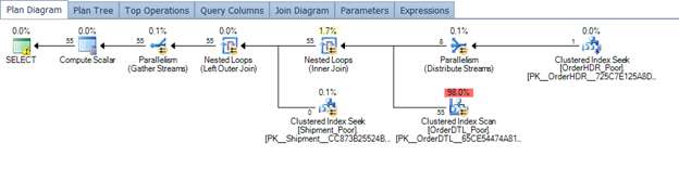
Figure 4 – Querying a poor design
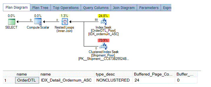
In order to tune this plan, an index would help the overall performance on ordernum in the order details table.
CREATE NONCLUSTERED INDEX IDX_ordernum_ASC
ON [dbo].[OrderDTL_Poor] ([ordernum])
INCLUDE ([item],[itemcost],[itemqty],[shipid])
GO
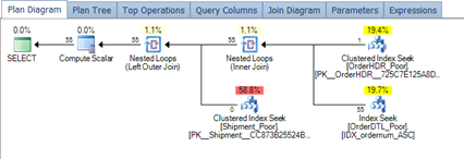
Figure 5 – Plan after tuning
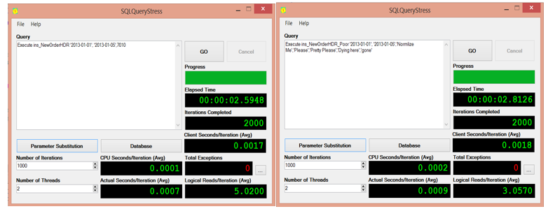
With the new plan after tuning with the indexing, the number of pages being pulled into the buffer are shown below in Figure 6. Overall, the page count is not high.
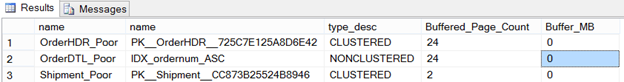
Figure 6 – Buffer review after tuning
This plan isn’t bad and will perform fairly well under normal conditions. Let’s compare this to the same procedure and the plan that is generated based on the design of the normalized tables.
CREATE PROCEDURE select_OrderDetailsByOrderNumv2 (@ordernum INT)
AS
SELECT
	hdr.ordernum,
	hdr.orderdate,
	dtl.item,
	dtl.itemcost,
	dtl.itemqty,
	CASE WHEN ship.ShipID IS NULL THEN 'Not Shipped'
	ELSE CAST(shipDate AS VARCHAR(12)) END [Ship Date]
FROM OrderHDR hdr
JOIN OrderDTL dtl ON hdr.ordernum = dtl.ordernum
LEFT JOIN Shipment ship ON dtl.ShipID = ship.shipID
WHERE hdr.ordernum = @ordernum
GO
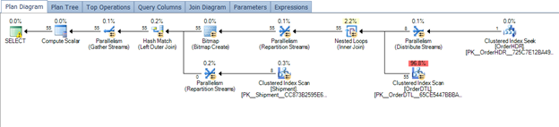
Figure 7 – normalizing and plan generated from same procedure
CREATE NONCLUSTERED INDEX IDX_Detail_Ordernum_ASC
ON [dbo].[OrderDTL] ([ordernum])
INCLUDE ([item],[shipID],[itemcost],[itemqty])
GO

Figure 8 – Plan after tuning
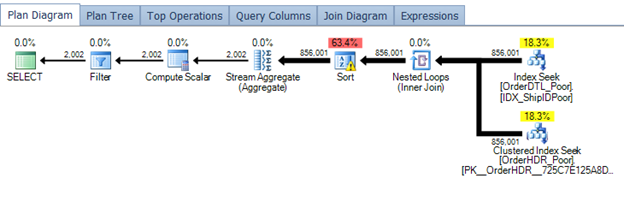
We do see a slight difference in the operational cost of the order header and detail tables. This is effectively due to the cost associated with the size. Looking at the buffer usage, we see a slightly lower number of pages from the header table. Given the header table is the one holding the most redundancy in the non-normalized design, this was expected.

Figure 9 – Review buffered page counts
Another example would be a common task – check if an order is shipped. To do this, in both cases we need to look at the detail table and the shipment table.
CREATE PROCEDURE sel_ShipDate (@ordernum INT)
AS
SELECT
	1
FROM OrderDTL_Poor dtl
INNER JOIN Shipment_Poor ship ON dtl.shipid = ship.shipID
WHERE dtl.ordernum = @ordernum
GO
From the above procedure, the following plan is generated and resulting buffer needs in page count.
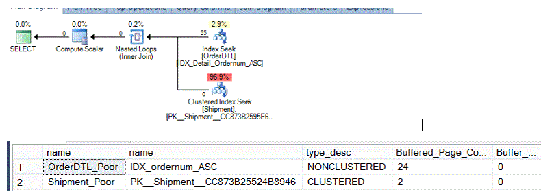
Looking at the normalized design and the same needs, the following procedure can be used and executed.
CREATE PROCEDURE sel_ShipDatev2 (@ordernum INT)
AS
SELECT
	1
FROM OrderDTL dtl
INNER JOIN Shipment ship ON dtl.shipid = ship.shipID
WHERE dtl.ordernum = @ordernum
GO
Resulting in the following plan and buffer needs as page counts.
As we can see, there isn’t a large difference. So far we’ve looked at queries and plans that are similar in resource consumption, other than a slight variance in pages pulled into the buffer. Let’s take a look at the order header table now. The order header table takes on a severe non-normalized factor. The first thing that is obvious is the customer data. In the poorly designed order header table, the customer data is not unique – it’s repeated and redundancy starts to creep in.
With the order header table, poor design and working towards normalization, we’ll start to see a larger impact to the IO requirements, equating to more CPU and buffer usage, from querying the table. Let’s take a typical example where a query is needed to return customers that have placed more than 3 orders, the number of orders they have placed, and only orders that have shipped will be acceptable. To perform this query, we would read both designs slightly differently.
Poor design – non-normalized
select
	hdr.customerName,
	count(*)
from OrderHDR_Poor hdr
join OrderDTL_Poor dtl on hdr.ordernum = dtl.ordernum
join shipment_Poor ship on dtl.shipid = ship.shipid
where dtl.shipid is not null
group by hdr.customerName
having count(*) > 3
Normalizing
select
	cust.contactName,
	count(*)
from OrderHDR hdr
join OrderDTL dtl on hdr.ordernum = dtl.ordernum
join shipment ship on dtl.shipid = ship.shipid
join Contact cust on hdr.customerID = cust.contactID
where dtl.shipid is not null
group by hdr.customerID,cust.contactName
having count(*) > 3
Both of these queries are easily tuned with indexing on ShipID. Further indexing could be done but we’ll look at indexing ShipID given it has the highest cost for both queries.
CREATE NONCLUSTERED INDEX IDX_ShipIDPoor
ON [dbo].[OrderDTL_Poor] ([shipID])
INCLUDE ([ordernum])
GO
Plan for the non-normalized design (note the sort operation due to poor statistics
CREATE NONCLUSTERED INDEX IDX_ShipID
ON [dbo].[OrderDTL] ([shipID])
INCLUDE ([ordernum])
GO
Now a plan for the more normalized design.
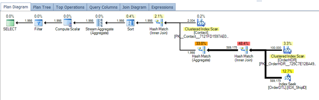
These two plans take on a very different path and overall impact to the resource utilization for the server. The first plan on the poor design, shows a small plan that is effectively performing two index seeks. This, in many eyes, would be seen as okay and may be skipped over in a performance troubleshooting situation. However, the overall execution time is 3062 milliseconds. Again, this may not seem like a major issue but if this query was used in a normal operation that caused an execution count of 300 and hour, we are looking at a potential bottleneck in performance. Poor statistics are also in play here and selectivity. Altering the statistics by updating would generate a different but still, not memory effective plan.
Looking at the second plan on the table designs that have been normalized more, the plan appears to be working better. Equating this to harder is not accurate though. The total execution time for the design that has been normalized more is 296 milliseconds. Looking at the plan, we see the sort operation is not coming in given the grouping now forced to the normalized table of Contact. Both queries could be tuned further, but this shows a good representation of a typical performance issue we can find ourselves facing from a poorly designed table structure and lack of normalization.
So what were the IO effects? The cause behind the poor performance of the design with little normalization was IO.
For the design that implemented more normalization, we pulled the following into the buffer.
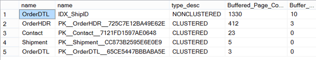
For the design that has little to no normalization
As we can see, the impact of these two designs and either normalizing or not, has a major impact on the overall IO needs relating to needs for the memory.
The normalized procedure to insert a header row takes more effort with a lookup to the contact table to ensure there isn’t a violation of the key constraint. The resources used in the insert and the page level, all equating to more IO, cause this to still be slightly more efficient though.
Summary
As shown, normalization is the basis of removing redundancy in a database. Although redundancy may not seem, at first, like a concept that could impact performance, we’ve learned today that even a small amount of redundant data in a few columns can impact a database’s resource needs, growth and scalability.
When designing OLTP or OLAP databases, take into account the data that will be stored. Manipulate the tables as you design and go through modeling practices with data that would represent the future, completed design. This will help identify needs for normalization or de-normalization, depending on which design you are working to accomplish.


